Digital & Embedded Systems

Tutorial 7 - Position Control of a Non-Holonomic System

This tutorial will demonstrate how to control a non-holonomic system. The system that will be discussed is the position control of a differential drive robot.

A non-holonomic system is a system where the number control variables, n, are less than the number of output variables, m. For the differential drive robot, there are two control variables, f' = [f'1,f'2], and three output variables, p' = [x',y',q'].

Coordinate Systems - Global vs. Local

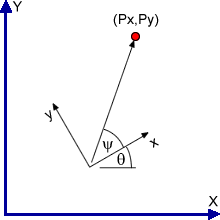
Before continuing, we will distinguish the difference between global and local coordinate systems and review the concept of homogeneous transformation matrices. Figure [1] illustrates two coordinate systems. The global coordinate system is plotted in blue, the local coordinate system is plotted in black, and a position coordinate is plotted in red.

Figure 1 - Global vs. Local Coordinate Systems

We can describe the location of any point in p, with respect to a base coordinate frame, by a [3x3] matrix, denoted here as T. This type of matrix is called a homogeneous transformation matrix and matrices of this type are used widely in robotics and computer graphics.

The a terms represent the approach vector, the n terms represent the normal vector and the d terms represent the distance vector. Notice that this vector is square and by examining the determinant

it follows that the T matrix is also invertible. Another, more compact, way to represent T is in the following form

where R is a [2x2] matrix representing the rotation components, and d is a [2x1] vector representing the displacement components. The 0 in the lower left corner has a bar to denote that it represents a [1x2] vector of zeros. The inverse of the T matrix can be shown to be equal to

So if the location in 3-space is defined by [x,y,q], then the cooresponding T and inv(T) matrices are

 

Differential Drive Kinematics

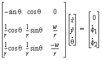
A differential drive is one of the simplest drive configurations in terms of geometry and complexity, therefore it is widely used for mobile robot applications. The kinematic equations for the differential drive are

The above equations can be written in matrix form as

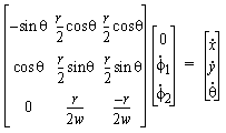
This equation is in the wrong form because we would like to calculate velocity based on individual wheel velocities. Remember that Ax = b therefore x = inv(A)b, so we must invert the A matrix. First, check that the determinant does not equal zero, which it does not.

After inversion, the resulting equation is

An important observation is that any point in the [x,y,q] space can be reached by controlling the inputs f. However, it is not all trajectories in the 3-space can be followed by the vehicle (any trajectory requiring the robot to move in a direction along the wheel axis is impossible). There are various approaches to solving this problem, including optimal control, sliding mode control, or other non-linear control laws, however we will take a simplier approach. By only allowing the robot to either turn about its midpoint or travel in a straight line, we can decouple the kinematic equations and realize a controllable system.

A rotation about the z-axis can be represented as

Similar to the rotation matrix, a tranlation along the x-axis can be represented as

As was stated above, in order to decouple the kinematic equations, we will only let the robot turn on its midpoint or travel in a straight line (in the x-direction in the robot's local coordinate system). Therefore, to move the robot to a new location, first the robot must turn so that the point lies directly in front and then drive a set distance to the location. This can be stated mathematically as

Equivently, we can describe the location, with respect to the global coordinate system, as a translation followed by a rotation. Mathematically this is expressed as

We have shown in the first section that these two descriptions are equivalent, therefore we can equate the two transformations. Notice that question marks are left in the rotational component of the resulting matrices because we are only concerned with position (x,y) and not orientation.

Now we have two equations with two unknowns which we can solve by

Now the y term represents the amount that the robot should turn about its midpoint, and the r term represents the forward distance the robot should travel.